End result

Requirements

Basic linear algebra knowledge. Understanding of javascript and basic 3D visualization.

Background

I recently started learning about robotics. I reached out to my network for some good book recommendations and looked at class curriculums and settled on two main texts: Modern Robotics and Probabilistic Robotics. For a more in-depth understanding of these concepts, please refer to one of these sources. But if you want to see the core of how I implemented a quick-and-dirty general IK solver, read on!

Modern Robotics begins with rigidbody dynamics and Inverse Kinematics. Some of the math seems daunting but it’s actually not that complicated when you start to think in code. One of the key concepts is the Homogeneous Transform Matrix. A homogeneous transform matrix (also called SE(3)) is a 4x4 matrix that contains rotation and position information. If you multiply A x B, the resultant matrix will be A translated and rotated by B.

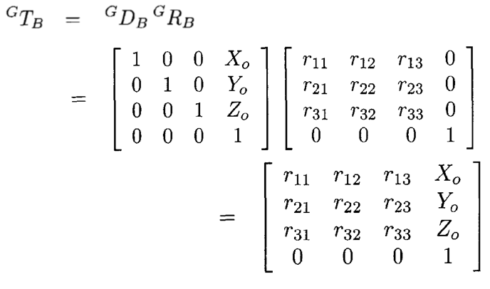
The “r”s in GRB control rotation. X0, Y0, and Z0 control translation. Different matrices control the rotation on different axes:

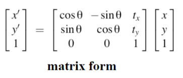
It looks like a lot, but we wil build up to it. For now let’s focus on 2D. A 2D transformation matrix looks like the form:

The 2D rotation matrix looks like this in code:

[
    [Math.cos(θ), -Math.sin(θ)],
    [Math.sin(θ), Math.cos(θ)]
]

We can pad it with the identity matrix to make it into a transformation matrix:

[
    [[Math.cos(θ), -Math.sin(θ), x],
    [Math.sin(θ), Math.cos(θ), y],
    [0, 0, 1]]
]

This matrix will translate any other transform matrix by x and y, then rotate it by θ. Try it yourself by hand. Multiply a vector at x = 2, y = 2 with a rotation of 0 degrees by some other transform matrix. Does the resulting vector make sense?

If we have an arm with length “r” that is rotating with an angle of theta, we can represent the coordinate position of the end of the arm (called the “end effector” like this:

    [[Math.cos(θ), -Math.sin(θ), r * Math.cos(θ)],
    [Math.sin(θ), Math.cos(θ), r * Math.sin(θ)],
    [0, 0, 1]]

The values of x and y are derived from polar coordinates. x = r * cos(θ), y = r * sin(θ). Notice that this is also the result of the operation:

[
    // pure rotation matrix
    let A = math.matrix([
        [Math.cos(θ), -Math.sin(θ), 0],
        [Math.sin(θ), Math.cos(θ), 0],
        [0, 0, 1]
    ])

    // pure translation matrix
    let B = math.matrix([
        [1, 0, r],
        [0, 1, 0],
        [0, 0, 1]
    ])

    // combine the rotation and translation!
    let C = math.multiply(A, B)
]

So this means we can represent any sequence of robot arm components with a sequence of transformation matrices. To limit confusion from now on I will refer to the parts of robot arms that move as “joints” and the rigid parts as “link”. In your own body your knees and elbows would be the joints, while your forearms and lower legs would be the links. There are also other joints like spherical joints (consider your hips and shoulders with ball and socket joints) and prismatic joints (think of a gantry in a CNC machine or 3D printer). This guide will only cover revolute joints.

So we have a way to start with the angles of every joint and calculate the position of the end effector. The next step is to figure out how we can do this in reverse. Pick an end-effector position and generate all of the arm angles that will get us there.

Robot Arms

Now that we understand the matrices, let’s look at an actual equation for a very basic robot arm:

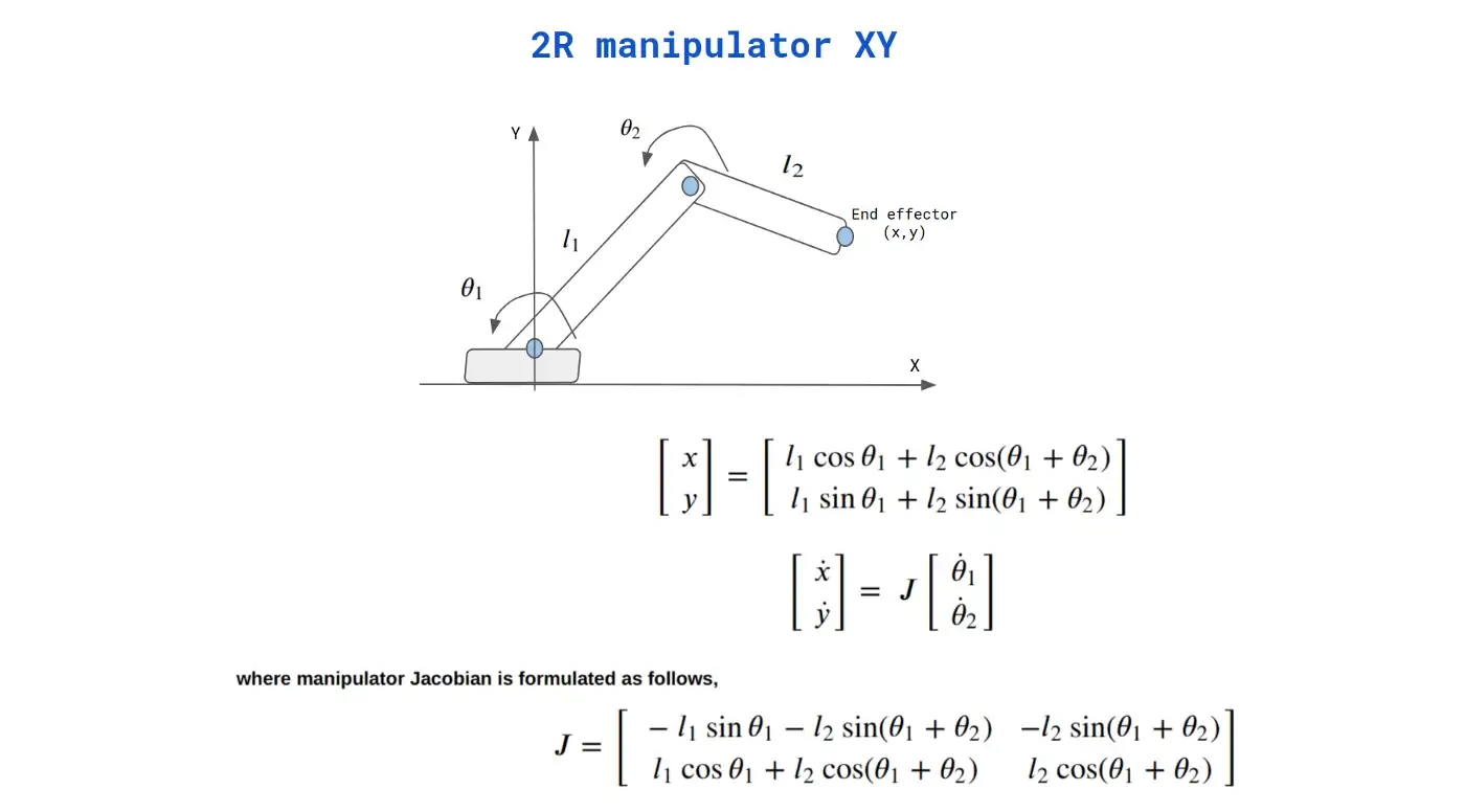
This matrix is actually just a pair of parallel equations. We can use basic algebra and trig to substitute and find out the solutions. This type of arm will typically have 2 solutions for any given end effector position, since the elbow can be bent at a negative or positive angle.

Stop and think how many “degrees of freedom” this robot has with respect to its joints– AKA how many variables are required to represent the state of the arm? Well it can rotate on two axes, so two. The two angles of the two joints. How many DOF does the end-effector have? Well we can represent any point in the plane in either polar (0, r) or cartesian (x, y) coordinates, so two DOF.

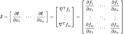
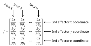
Ok quick detour. There is a special matrix called a Jacobian which is just a matrix of partial derivatives. See the df/dx in the image below? Each of those items is basically saying “how much does each output variable change according to a change in some input variable?”. In the case of our robot arm, we could say the x coordinate of the end effector changes by some amount if we change the first arm’s angle by some value, which would be dx/d01. A lot of Inverse Kinematics solvers use this Jacobian matrix directly. We wont be doing that. If you are interested in learning more, look up “Jacobian Transpose” and “Jacobian Pseudoinverse”.

If the degrees of freedom of the arm is the same as the degrees of freedom of the end-effector then our Jacobian is square. Square matrices are invertible. What this means basically is that you can solve a “non-redundant” inverse kinematics problem analytically. So long as you can calculate that inverse matrix, you can figure out what joint position you need.

But what if we want to solve for a more complicated arm with infinite solutions, or 100 joints? The Jacobian becomes a rectangle! We can’t invert rectangles! We can no longer solve algebraically in that case. We now have to treat this problem like an optimization problem.

There are lots of ways to solve IK as an optimization problem. This page has a lot of really good examples. I initially went with gradient descent.

Gradient Descent

Gradient Descent is not a difficult concept by itself, I will try to explain it with as little math as possible. You will just need to remember the definition of a derivative:

Imagine that you are blindfolded on top of a large hill or mountain, and you need to find your way to the bottom of it. One possibility would be to take a step north (+X) and a step east (+Y). If your step north is downhill, then move north. If your step east is downhill, then move east. If your step north is uphill, then move south. If your step east is downhill, then move west. At each step you are measuring the partial derivative of f(x,y) = z “How much elevation (z) will I gain for a small change in x?”

After enough of these steps, you should reach the bottom of the mountain. The “gradient” in gradient descent is just a vector holding the partial derivatives. Basically a map to tell you which directions will bring you down the mountain for any given step.

Notice how one of the balls in this gif gets stuck on a little divot on top of the hill. This is called a “local minimum”. These can be tricky to escape. There are some methods that help escape these traps like momentum, which carries over between steps and gives you enough “oomph” to roll out of these divots. There are also algorithms like Evolutionary Algorithms which have a random component that helps them “jump” out of these local minimum. For now lets KISS and just focus on gradient descent.

Implementation of a Robot Arm in 2D

Gradient Descent algorithm

By taking a lot of little steps in the right direction, we can move our robot arm to the target destination!

Related Video

(visualization is done in HTML canvas)

To find the partial derivatives at each angle and calculate the gradient is pretty simple.

1. Start with some θ
2. Find the position of the end of the arm for all the angles
3. Find the difference between actual end effector position and target end effector position. This is the “Loss” for the current arm configuration. (Loss1)
4. Nudge θ by some small number, d, like 0.00001. This is θ’
5. Find the position of the end effector for all angles including this new angle, θ’
6. Find the difference between this new end effector position and target end effector position. This is Loss2
7. Find (Loss2 - Loss1) / d

This works out to the difference in Loss for a given difference in the angle θ Or dF/dθ

Computing this for every joint in the arm will give us a gradient. Then all we need to do is subtract this gradient from the vector of arm angles, and it will bring us closer to the target position.

In code this looks like:

// this.thetas and this.radii are the current joint angles and link lengths for the arm

const d = 0.00001

for (let i = 0; i < this.thetas.length; i++) {
    const dTheta = this.thetas[i] + d
    const radius = this.radii[i]

    // generate the matrix for the new angle
    const dMat = generateMatrix2D(dTheta, radius)

    // generate the new arm position
    const deltaEndEffector = math.multiply(math.multiply(this.forwardMats[i], dMat), this.backwardMats[i+2])

    let dLoss = (this.calculateLoss(deltaEndEffector, i, dTheta, dMat) - this.loss) / d

    this.thetas[i] -= dLoss
}

I won’t code the full solution in this tutorial since it’s just supposed to give a basic overview, but the code for a 2D arm with Gradient Descent is here.

Matrices and Optimization

For all my matrix math I used math.js. For each section of the arm (remember a joint and a link correspond to a single transform matrix) we can generate a matrix with the following code:

function generateMatrix2D(theta, radius) {

    const cos = Math.cos(theta)
    const sin = Math.sin(theta)

    return math.matrix([
        [cos, -sin, radius * cos],
        [sin,cos, radius * sin],
        [0, 0, 1]
    ])

}

A quick detour into matrix algebra. These transform matrices are associative, meaning that A x B x C = (A x B) x C. But they are not commutative. Meaning A x B x C != A x C x B.

This is useful for representing our matrices internally. If an arm has an origin O and 5 segments A, B, C, D, E. Then we would represent the end-effector F with the equation:

O x A x B x C x D x E = F

For our gradient calculations, if we want to find dF/dθ for θc, we would want to calculate:

O x A x B x C' x D x E = F'

By caching our intermediate matrices, we can reduce this calculation to just 2 matrix operations instead of 5.

(O x A x B) x C' x (D x E) = F'

(O x A x B) is pre-computed in a forward pass, while (D x E) is calculated in a backward pass.

This is similar to the leetcode Product of Array Except Self problem.

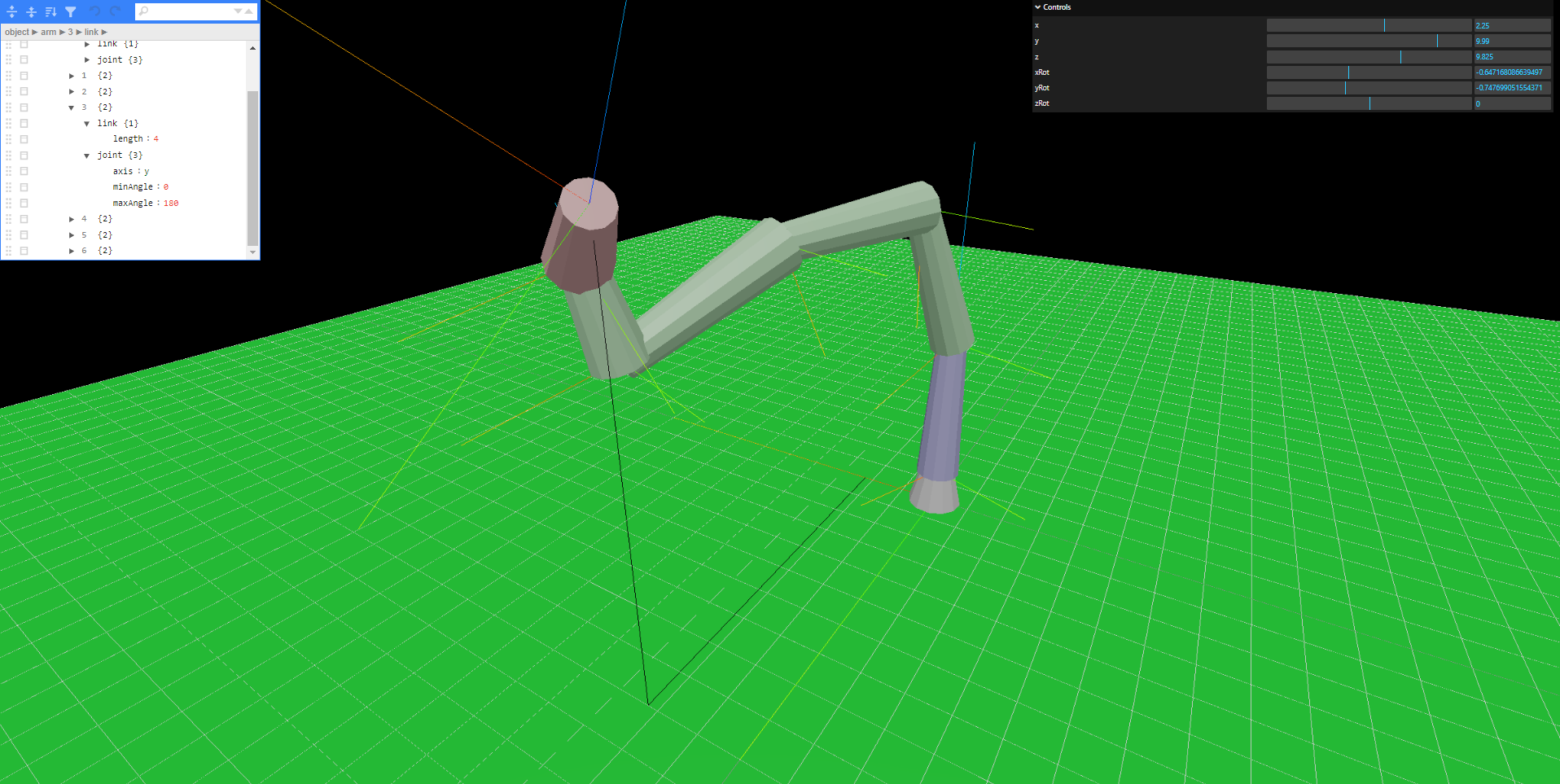
Implementation of an Arm in 3D

The matrix representation and gradient descent are the core of our implementation. So once we have a solver working in 2D, it should be trivial to implement it in 3D. In 2D we can only rotate along the axis that runs out of the 2D plane (the normal). In 3D we need to specify which axis we are rotating around. There are different rotation matrices for each axis. So in addition to the joint angle and link length of an arm segment, we will also need to specify the axis of rotation.

/**
 * Constraints: only handles one-axis rotation at a time. Radius is locked to z-axis
 * @param {number} theta amount to rotate by
 * @param {string} axis axis to rotate around. Must be x, y or z 
 * @param {number} radius length in z-axis
 */
export function mat4(theta, axis, radius) {

    const tMat = tMat3D(0, 0, radius)
    const rMat = rMat3D(theta, axis)

    return math.multiply(tMat, rMat)

}

To create a matrix4, I specify an arm radius to generate the translation matrix, and a theta + axis to generate one of three types of rotational matrices. Multiplying them gives a matrix which will rotate the frame of reference, then translate along that new rotated axis.

You can see more details in Geometry.js

Other than having different matrices, our solver logic is basically unchanged. The large changes happen in visualization. Arm3D.js

We create an array of arm segments and update them using a Matrix4 every frame. The Matrix4 for math.js and Three.js is represented differently, so it’s necessary to write a helper function to convert between the two types.

Conclusion

You’re done! This is probably the most basic solver that you can implement. But from here it’s fairly easy to add complexity. You can add joint constraints that prevent joints from bending too far in a given direction. You can add self-intersection constraints using bounding boxes, and obstacle avoidance using many different methods, path planning, etc. You can also implement different solvers and try out different optimization algorithms.